From Łukasz Graczykowski
(Difference between revisions)
|
|
| Line 4: |
Line 4: |
| | Using the least-squares method, fit to the data polynomials of varying degrees <code>n=0..5</code>. | | Using the least-squares method, fit to the data polynomials of varying degrees <code>n=0..5</code>. |
| | | | |
| - | * Please read data from the following [http://www.if.pw.edu.pl/~lgraczyk/KADD2016/lab11/dane.dat file]. They come from the experiment of elastic collisions of negatively charged K mesons (kaons) with protons, at constant K meson energy. In the first column there are values of the cosine of the scattering angle in the rest mass reference frame, in the second column is the corresponding number of collisions. As errors please assume the square root of the number of observations. The degree of fitted polynomial allows to calculate sge Jeżeli otrzymany rozkład ma postać wielomianu, to wyznaczenie jego stopnia umożliwia wyznaczenie spinowych liczb kwantowych występujących stanów pośrednich ("Analiza danych", S.Brandt, Przykład 9.2.). | + | * Please read data from the following [http://www.if.pw.edu.pl/~lgraczyk/KADD2016/lab11/dane.dat file]. They come from the experiment of elastic collisions of negatively charged K mesons (kaons) with protons, at constant K meson energy. In the first column there are values of the cosine of the scattering angle in the rest mass reference frame, in the second column is the corresponding number of collisions. As errors please assume the square root of the number of observations. The degree of fitted polynomial allows to calculate the spin quantum numbers of intermediate stages ("Analiza danych", S.Brandt, Przykład 9.2.). |
| | | | |
| - | * Proszę zaimplementować funkcję realizującą procedurę dopasowania metodą najmniejszych kwadratów. W tym celu należy wykorzystać wzory (ich wyprowadzenie znajduje się w [http://www.if.pw.edu.pl/~lgraczyk/KADD2019/Wyklad12-2019.pdf wykładzie 12] (od slajdu 22) oraz w [http://www.if.pw.edu.pl/~majanik/files/wiel.ps instrukcji]) - '''proszę dokładnie przeczytać tę instrukcję - zadanie robimy zgodnie z nią''': | + | * Please implement the function realizing the least-squares method. Use formulas from the lecture (ich wyprowadzenie znajduje się w [http://www.if.pw.edu.pl/~lgraczyk/KADD2022/Wyklad11-2022.pdf Lecture 12] and from the unstruction [http://www.if.pw.edu.pl/~majanik/files/wiel.ps instrukcji]) - '''please carefully read the instruction - all the steps should follow the instruction''': |
| | | | |
| | [[File:wzor1_new_asd.png]] | | [[File:wzor1_new_asd.png]] |
| Line 20: |
Line 20: |
| | [[File:wzor89.png]] | | [[File:wzor89.png]] |
| | | | |
| - | ''Komentarz'': szukamy minimum funkcji M (odpowiednik statystyki chi-kwadrat), wartości <code>t_{j}</code> to cosinusy kąta rozproszenia (pierwsza kolumna pliku), wartości <code>y_{j}</code> to liczby obserwacji (druga kolumna). Estymatory <code>x</code> to poszukiwane współczynniki wielomianu. | + | ''Comment'': we search from a minimum of M function (equivalent of chi-squared statistics), values <code>t_{j}</code> are the cosine scattering functions (first column from the file), values <code>y_{j}</code> are the observations numbers (second column). Estimators <code>x</code> are the searched parameters (coefficients) of the polynomial. |
| | | | |
| - | Przykładowy nagłówek funkcji:
| + | Example function definition: |
| - | // Funkcja zwraca wartosc funkcji M | + | // Function returns M |
| - | // parametry: | + | // parameters: |
| - | // st - stopien dopasowanego wielomianu | + | // st - degree of the polynomial |
| - | // n - liczba pomiarow | + | // n - number of measurements |
| - | // tj - tablica cosinusow kata rozproszenia | + | // tj - array of cosine of scattering angles |
| - | // yj - wyniki pomiarow | + | // yj - measurement results |
| - | // sigmaj - bledy pomiarow | + | // sigmaj - measurement errors |
| - | // wsp - tablica do ktorej nalezy wpisac wartosci wyznaczonych wspolczynnikow ([[File:wzor10.png]]) | + | // wsp - array in which we need to save estimated coefficients ([[File:wzor10.png]]) |
| - | // bswp - tablica do ktorej nalezy wpisac bledy wyznaczonych wspolczynnikow (pierwiastki kwadratowe z elementów diagonalnych macierzy [[File:wzor11.png]]) | + | // bswp - array in which we need to save estimated coefficient errors (square roots of the diagonal elements of the matrix [[File:wzor11.png]]) |
| - | double dopasuj (int st, int n, double *tj, double *yj, double *sigmaj, double *wsp, double *bwsp); | + | double fit (int st, int n, double *tj, double *yj, double *sigmaj, double *wsp, double *bwsp); |
| | | | |
| - | Do zaimplementowania powyższych wzorów wygodnie jest skorzystać z klasy [http://www.slac.stanford.edu/comp/unix/package/cernroot/30106/TMatrixD.html TMatrixD]. Przykłady jej użycia:
| + | To implement the formulas please use the class [http://www.slac.stanford.edu/comp/unix/package/cernroot/30106/TMatrixD.html TMatrixD]. Examples: |
| | | | |
| | // utworzenie macierzy o wymiarach n x m | | // utworzenie macierzy o wymiarach n x m |
| Line 51: |
Line 51: |
| | macierz->Invert(); | | macierz->Invert(); |
| | | | |
| - | * Proszę zinterpretować otrzymane dopasowania przeprowadzając test chi-kwadrat (korzystając z wyznaczonej wartości funkcji M). Należy określić stopień wielomianu, dla którego dopasowanie jest najlepsze oraz wyznaczyć najmniejszy stopień wielomianu, którego nie możemy odrzucić. Proszę wypisać wartości wyznaczonych współczynników wielomianu. | + | * Please interpret the resulting fitting by performing a chi-squared test (using the M functions). Please state which degree of the polynomial fits data best (what is the lowest degree of the polynomial, for which we do not reject the null hypothesis) |
| | | | |
| - | == Wynik == | + | == Result == |
| | | | |
| | [[File:mnk_2.png]] | | [[File:mnk_2.png]] |
Latest revision as of 11:48, 23 May 2022
Zadanie
Least-squares method (5 pkt.)
Using the least-squares method, fit to the data polynomials of varying degrees n=0..5.
- Please read data from the following file. They come from the experiment of elastic collisions of negatively charged K mesons (kaons) with protons, at constant K meson energy. In the first column there are values of the cosine of the scattering angle in the rest mass reference frame, in the second column is the corresponding number of collisions. As errors please assume the square root of the number of observations. The degree of fitted polynomial allows to calculate the spin quantum numbers of intermediate stages ("Analiza danych", S.Brandt, Przykład 9.2.).
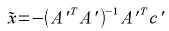
- Please implement the function realizing the least-squares method. Use formulas from the lecture (ich wyprowadzenie znajduje się w Lecture 12 and from the unstruction instrukcji) - please carefully read the instruction - all the steps should follow the instruction:
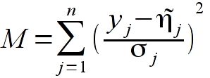
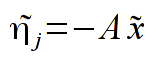
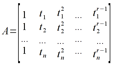
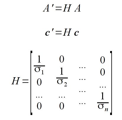
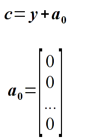
Comment: we search from a minimum of M function (equivalent of chi-squared statistics), values t_{j} are the cosine scattering functions (first column from the file), values y_{j} are the observations numbers (second column). Estimators x are the searched parameters (coefficients) of the polynomial.
Example function definition:
// Function returns M
// parameters:
// st - degree of the polynomial
// n - number of measurements
// tj - array of cosine of scattering angles
// yj - measurement results
// sigmaj - measurement errors
// wsp - array in which we need to save estimated coefficients ( )
// bswp - array in which we need to save estimated coefficient errors (square roots of the diagonal elements of the matrix
)
// bswp - array in which we need to save estimated coefficient errors (square roots of the diagonal elements of the matrix 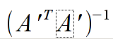 )
double fit (int st, int n, double *tj, double *yj, double *sigmaj, double *wsp, double *bwsp);
)
double fit (int st, int n, double *tj, double *yj, double *sigmaj, double *wsp, double *bwsp);
To implement the formulas please use the class TMatrixD. Examples:
// utworzenie macierzy o wymiarach n x m
TMatrixD *macierzA = new TMatrixD(n,m);
// dostep do elementu o indeksach i,j macierzy macierzA, np.:
(*macierzA)(i,j) = 1;
// mnozenie macierzy: macierzA = macierzB macierzC
TMatrixD *macierzA = new TMatrixD(*macierzB, TMatrix::kMult, *macierzC);
// transponowanie macierzy
TMatrixD *macierzAt = new TMatrixD(TMatrix::kTransposed,*macierzA);
// odwracanie macierzy
macierz->Invert();
- Please interpret the resulting fitting by performing a chi-squared test (using the M functions). Please state which degree of the polynomial fits data best (what is the lowest degree of the polynomial, for which we do not reject the null hypothesis)
Result
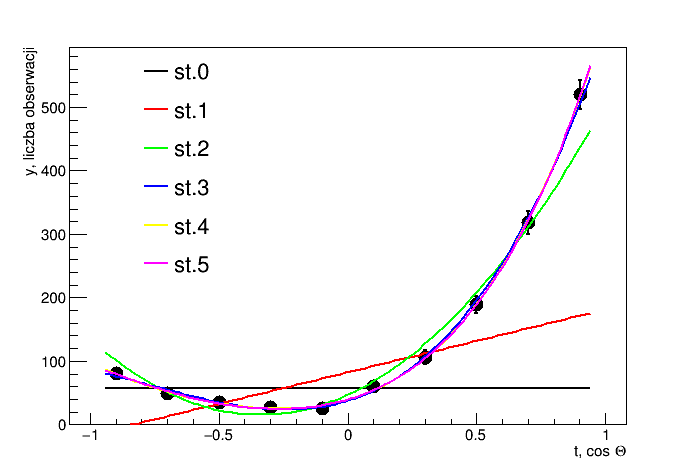
Output:
 Dopasowanie wielomianem stopnia 0
 M = 833.548
 x0 = 57.8452 +- 2.4051
 Liczba stopni swobody=9
 Kwantyl=21.666
 Poziom istotnosci=0.01
 Stopien 0: odrzucamy
 Dopasowanie wielomianem stopnia 1
 M = 585.449
 x0 = 82.6551 +- 2.87498
 x1 = 99.0998 +- 6.29159
 Liczba stopni swobody=8
 Kwantyl=20.0902
 Poziom istotnosci=0.01
 Stopien 1: odrzucamy
 Dopasowanie wielomianem stopnia 2
 M = 36.4096
 x0 = 47.267 +- 3.24753
 x1 = 185.955 +- 7.30235
 x2 = 273.612 +- 11.6771
 Liczba stopni swobody=7
 Kwantyl=18.4753
 Poziom istotnosci=0.01
 Stopien 2: odrzucamy
 Dopasowanie wielomianem stopnia 3
 M = 2.84989
 x0 = 37.949 +- 3.62403
 x1 = 126.546 +- 12.5894
 x2 = 312.018 +- 13.4278
 x3 = 137.585 +- 23.7499
 Liczba stopni swobody=6
 Kwantyl=16.8119
 Poziom istotnosci=0.01
 Stopien 3: akceptujemy
 Dopasowanie wielomianem stopnia 4
 M = 1.68602
 x0 = 39.6179 +- 3.94036
 x1 = 119.102 +- 14.3563
 x2 = 276.49 +- 35.5643
 x3 = 151.91 +- 27.2096
 x4 = 52.5999 +- 48.7566
 Liczba stopni swobody=5
 Kwantyl=15.0863
 Poziom istotnosci=0.01
 Stopien 4: akceptujemy
 Dopasowanie wielomianem stopnia 5
 M = 1.66265
 x0 = 39.8786 +- 4.29351
 x1 = 121.384 +- 20.7054
 x2 = 273.188 +- 41.6103
 x3 = 136.571 +- 103.954
 x4 = 56.8995 +- 56.2858
 x5 = 16.7294 +- 109.424
 Liczba stopni swobody=4
 Kwantyl=13.2767
 Poziom istotnosci=0.01
 Stopien 5: akceptujemy


