KADD 2022 Laboratorium 7 EN

From Łukasz Graczykowski

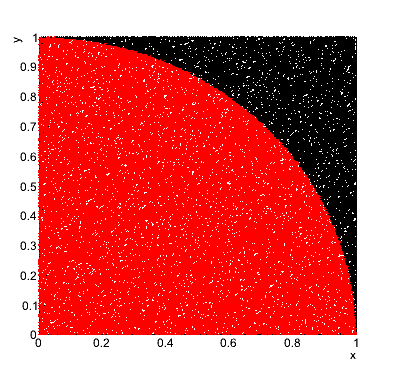
Exercise

Part one: estimation of the Pi (1 pkt.)

Please write a function which estimates the number Pi with the von Neumann (it is arguably one of the most simple examples of the use-case of a Monte Carlo method). In order to calculate the Pi, we randomly generate two numbers x and y from the uniform distribution [0,1] and we check whether the pair falls within the circle of the radius equal to 1. Next, by calculating the ratio of accepted pairs to all of them, you approximate the ratio of areas of the circle to the rectangle. By performing such a random generation, calculate the Pi number. In addition, draw the graph of the resulted points inside and outside the circle:

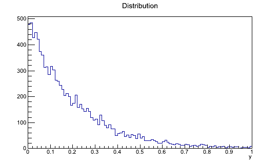
create two objects of type TGraph and fill one of them with accepted pairs (x,y), the second one with rejected pairs. Both plots draw on one canvas,
in addition, you can create a TH1D object and fill it with accepted values of x. It will be a distribution of the circle.

Part two: generation of pseudo random numbers from a any probability distribution using the acceptance rejection method of von Neumann (3 pkt.)

The transformation method used a week ago has limited applications. You can do this when the analytical form of the cumulative function and its inverse function are known. The von Neumann method of generation of pseudo random numbers will work when you know only the g(y) distribution, but the drawback is that you have to generate two numbers, now one. This method will also work if the g(y) function is not a proper probability distribution (it even does not need to be normalized - every function you can always normalize). This allows for a very broad application of the von Neumann method - also to calculate definite integrals, when their analytical form does not exist. This is a typical example of a Monte Carlo method.

Please prepare thee very similar functions taking as argument an object of type TF1. The arguments should be the function g and the range [min,max]:

double generateVonNeumann(TF1 *g, double min, double max) - function returning a generated pseudo random number from distribution g(y),
double efficiencyVonNeumann(TF1 *g, double min, double max, int n) - function returning the efficiency of the von Neumann method for a given g(y) function and the number of generations n,
double integra;VonNeumann(TF1 *g, double min, double max, int n) - function returning the definite integral (area under the curve) from function g(y) in the range [min,max] with the number of generations n.

Part three: acceptance rejection method of von Neumann with the helper function (1 pkt.)

In order to improve the efficiency of the von Neumann function, we can limit the area of random points generation with the use of a helper function. In that case we can generate one number from the pair from the s(y) helper function, instead of a uniform distribution:

double integralVonNeumannWithHelper(TF1 *g, TF1 *s, double min, double max, int n, double &wydajnosc) - returns the definite integral of the function g(y) in the range [min,max] for a given number of generations n. In addition, the function should take as an argument through a reference (because in C/C++ any function can return only one quantity).

The function s(y) we choose always in a way it is above the function g(y) and so that you can easily generate a random number from the s(y) distribution (i.e. by applying the transformation of the inverse cumulative distribution, like last time).

All calculations please fo for the following function:

Attention

Read carefully Lecture 5 link slides 9-17
To generate numbers from the uniform distribution, use function Uniform from class TRandom OR the generator written last time
Remember, always accept points below the curve to all generated points.
As a helper function we will use a linear function.
In the case of integration using a helper function, we always choose it in such a way that it is possible to generate the number from its distribution in an easy way (by inverting the cumulative distribution function) - in other words, we convert the rectangle (two uniform distributions) to another area inside which we draw (we must be able to draw numbers from this area)
Quadratic function and its inverse function:

Metoda Monte Carlo - Wikipedia.
Wykład 5

Results

Part one

Output:

 The Pi number equals: 3.14392

Parts two and three