From Łukasz Graczykowski
Exercise
Part one: linear congruent generator of pseudorandom numbers (1 pkt.)
Please write a generator of pseudorandom numbers and save generated numbers into a file.
The generator should be based on the following formula:
x[j+1] = (g*x[j] + c) mod m.
This generator is called LCG - linear congruent generator. Providing the first (beginning) number x[0] defines the whole series, which is periodic. The period depends on the parameters and under certain conditions it reaches maximum value of m. These conditions are:
-
c and m do not have joint divisors,
-
b = g-1 is a multiply of every prime number p, which is a divisor of a number m,
-
b is a multiply of 4 if n is also a multiply of 4.
For simplicity we can uuse c = 0, and in that case we get a multiplicative generator (MLCG).
- Value of
g and m should be easy to modify in the program.
The result of the macro execution should be a file with the name name.dat containing a series of generated numbers for a given set of parameters. The macro should be executed three times, resulting in three files: random1.dat, random2.dat, random3.dat, for the following parameters, respectively:
-
m=97 and g=23,
-
m=32363 and g=157,
-
m=147483647 and g=16807.
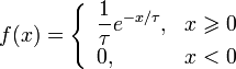
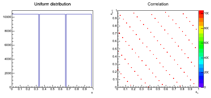
Second part: spectral test (1 pkt.)
Please perform a spectral test to see what is the quality of the generator. In order to do so please draw plot on the (x[n], x[n+1]) points from generated numbers. The obtained graph will show a spectral pattern of the generator - hence the name of the test.
If the points are distributed uniformly, the test can be judged good. If they show a certain periodic pattern - the test doesn't work properly. Of course, for the position of the points what maters are the parameters g and m.
- In order to draw spectral test, please use
TH2D.
As a result, we should have three spectral tests.
Third part: generation of pseudorandom numbers based on transformation of a uniform distribution (3 pkt.)
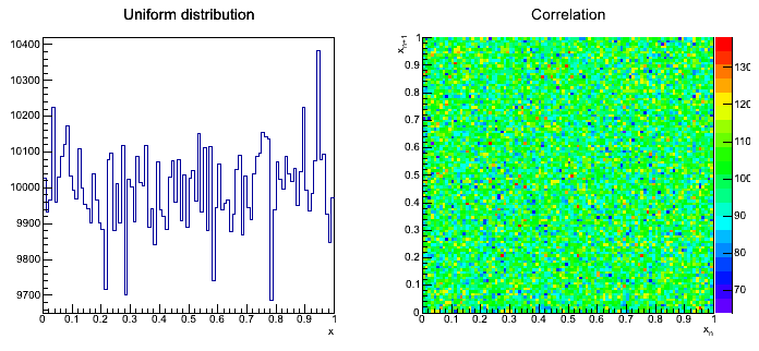
Each function of the random variable is also a random variable. What is the probability distribution of a random variable Y, if the probability distribution of X, f(x), is known. We assume, that the probability g(y)dy is equal to f(x)dx, where dx equals dy. The condition is of course fulfilled for (infinitely) small dx. What results from this is the following:
g(y) = dx/dy f(x)
Now, if we assume that the probability density f(x) equals 1 in the range 0<=x<=1 and f(x) = 0 for x<= 0 and x>1, then the above formula we can rewrite in the following form:
g(y)dy = dx = dG(y),
where G(y) is a cumulative distribution of the random variable Y. After integration this gives us:
x = G(y) => y = G^-1(x).
If the random variable X has a uniform distribution between 0 and 1 and we know the inverse function G^-1(x) then the function g(y) describes the probability distribution of the random variable Y.
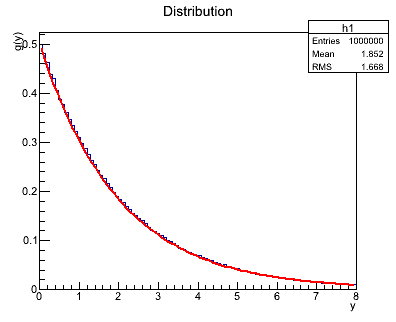
By using this method please generate 10000 numbers from the distribution:
For tau = 2:
- Generate 10000 numbers from the distribution from 0 to 1 using a generator from the first part (save in the file values of xn with a macro from the first file, in order to read them by a macro from the second part.).
- Analytically (on the piece of paper)calculate the cumulative distribution of this formula, then you need to invert it. (1 pkt.)
- Generate a distribution
f(x) - putting generated values into a histogram - korzystając z: (1 pkt.)
- numbers generated before and read from files
random1.dat, random2.dat, random3.dat,
- standard generator implemented in ROOT, i..e
gRandom->Uniform(1) (the object gRandom exists in the default instance of ROOT, you can also create it by using TRandom objects via a standard way by using a constructor - link).
- Draw on a single plot the histogram (normalized) and the theoretical function
f(x) (TF1 object). (1 pkt.)
Attention
- Read carefully the Lecture 4 (link), especially slids 6 and 8-25
- At the beginning, before random number generation, we need to set the first number from the series x0 (so called "seed"). If we want that every time the random numbers are different, we can set the seed from the system clock:
x0 = time(NULL);
- PArameters of the histograms shown below:
 TH1D *hUniform = new TH1D("hUniform","Uniform distribution",100,0,1);
 TH2D *hCorr = new TH2D("hCorr","Correlation",100,xmin,xmax,100,0,1);
- Number of random number generations:
const int N = 1000000;
- Example of reading from the text file:
ifstream ifile;
ifile.open("dane.dat");
double val;
while(ifile>>val)
{
  cout<<val<<endl;
}
ifile.close();
- Example of writing to the text file:
ofstream ofile;
ofile.open("dane.dat");
for(int i=0;i<N;i++)
  ofile<<val<<endl;
}
ofile.close();
Results
Example distribution for parameters:
Example transformation of a uniform distribution: