From Łukasz Graczykowski
(Difference between revisions)
|
|
| Line 1: |
Line 1: |
| - | == Zadanie == | + | == Exercise == |
| - | ''Część pierwsza'': '''Rozkład chi-kwadrat''' (3 pkt.) | + | ''Part one'': '''Chi-squared distribution''' (3 pkt.) |
| | | | |
| - | Napisać skrypt rysujący wykres rozkładu chi-kwadrat oraz jego dystrybuanty dla różnych wartości liczby stopni swobody: <code>n=1..20</code>.
| + | Write a script which will draw the chi-squared probability distribution and it's cumulative distribution for number of degrees of freedom in the range: <code>n=1..20</code>. |
| | | | |
| - | ''Część druga'': '''Dopasowanie funkcji Gaussa''' (2 pkt.) | + | ''Part two'': '''Fitting of the Gaussian function''' (2 pkt.) |
| | | | |
| - | Napisać skrypt dokonujący splotu n rozkładów jednostajnych. Liczbę n należy wyznaczyć jako najmniejszą liczbę dodanych rozkładów, dla której wartość chi2/ndf, obliczona na podstawie dopasowania funkcji Gaussa (wykorzystując gotowe funkcje klasy TF1 - używamy funkcji <code>Fit</code>) jest mniejsza od 1.0.
| + | Write a script which will perform a convolution of n uniform distributions. The value of n compute as a minimal number of convolutions, for which the value of chi2/ndf, calculated from the fit of the Gaussian function is lower than 1.0 (we use the method <code>Fit</code> from the TF1 class). |
| | | | |
| - | == Uwagi == | + | == Attention == |
| - | * Przechodzimy do '''drugiej części''' naszego przedmiotu - do tej pory zajmowaliśmy się własnościami rozkładów prawdopodobieństwa, teraz będziemy się zajmować szukaniem parametrów rozkładów prawdopodobieństwa (czyli '''estymacją''') na podstawie skończonej próby losowej (np. przeprowadzonego eksperymentu) | + | * We move to the '''second part''' of our class - until now we have considered only properties of the probability distributions. Now we will move to the methods of finding the parameters (estimation) of those distributions from the random sample (experiment). |
| - | * Czytamy dokładnie '''Wykład 8''' [http://www.if.pw.edu.pl/~lgraczyk/KADD2019/Wyklad8-2019.pdf link] - zwłaszcza slajdy dotyczące pobierania próby losowej z rozkładu normalnego (22-27) - najlepiej jednak przeczytać cały wykład, łącznie z wyjaśnieniem czym są estymatory i dlaczego rozkład chi-kwadrat jest taki ważny. Można również przeczytać '''Wykład 7''' [http://www.if.pw.edu.pl/~lgraczyk/KADD2019/Wyklad7-2019.pdf link] - slajdy od 27 do końca (w zasadzie to samo co Wykład 8, tylko z wyprowadzeniami) | + | * We read '''Lecture 9''' [http://www.if.pw.edu.pl/~lgraczyk/KADD2022/Wyklad9-2022.pdf link] - especially slides about the chi-squred distribution (22-27) - the best is to read the about the estimators. |
| - | * W części pierwszej do rozkładu chi-kwadrat należy zaimplementować wzór ze slajdu 24 - współczynnik '''k''' zawiera fumkcję gamma (<code>TMath::Gamma</code>) | + | * In the first part for chi-squared distribution we used the gamma function from (<code>TMath::Gamma</code>) |
| - | * W części drugiej wykonujemy n rozkładów jednorodnych i wynikowy histogram dopasowujemy funkcją Gaussa - powinna to być pętla (np. <code>while</code> albo <code>do-while</code>), którą przerywamy w momencie, gdy wartość statystyki testowej chi-kwadrat (X^2) dzielona na liczbę stopni swobody (NDF) jest mniejsza od 1. Do obliczania X^2 oraz NDF są odpowiednie funkcje w klasie TF1 (nie robimy tego ręcznie) | + | * In the second part we perform n convolutions of uniform distributions and the resulting histogram should be fitted with the Gaussian function - it should be a loop (i.e. <code>while</code> or <code>do-while</code>), which we break when the value of the test statistics chi-squared (X^2) divided by the number of degrees of freedom (NDF) is lower than 1. To calculate X^2 and NDF there are appropriate methods in the TF1 class |
| | | | |
| - | == Wynik == | + | == Result == |
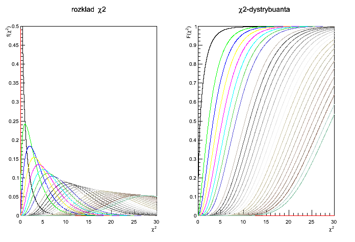
| - | '''Rozkład chi-kwadrat''' | + | '''Chi-squared distribution''' |
| | | | |
| | [[File:lab9_2.png]] | | [[File:lab9_2.png]] |
| | | | |
| - | '''Dopasowanie funkcji Gaussa''' | + | '''Fit of the Gaussian function''' |
| | | | |
| | [[File:lab9_splot.png]] | | [[File:lab9_splot.png]] |
| | | | |
| - | Output (przykładowy):
| + | Result (example): |
| - | liczba splecionych rozkladow jednostajnych = 9 | + | number of convoluted distributions = 9 |
| | chi2/ndf = 55.724/59 = 0.944475 | | chi2/ndf = 55.724/59 = 0.944475 |
Latest revision as of 11:09, 9 May 2022
Exercise
Part one: Chi-squared distribution (3 pkt.)
Write a script which will draw the chi-squared probability distribution and it's cumulative distribution for number of degrees of freedom in the range: n=1..20.
Part two: Fitting of the Gaussian function (2 pkt.)
Write a script which will perform a convolution of n uniform distributions. The value of n compute as a minimal number of convolutions, for which the value of chi2/ndf, calculated from the fit of the Gaussian function is lower than 1.0 (we use the method Fit from the TF1 class).
Attention
- We move to the second part of our class - until now we have considered only properties of the probability distributions. Now we will move to the methods of finding the parameters (estimation) of those distributions from the random sample (experiment).
- We read Lecture 9 link - especially slides about the chi-squred distribution (22-27) - the best is to read the about the estimators.
- In the first part for chi-squared distribution we used the gamma function from (
TMath::Gamma)
- In the second part we perform n convolutions of uniform distributions and the resulting histogram should be fitted with the Gaussian function - it should be a loop (i.e.
while or do-while), which we break when the value of the test statistics chi-squared (X^2) divided by the number of degrees of freedom (NDF) is lower than 1. To calculate X^2 and NDF there are appropriate methods in the TF1 class
Result
Chi-squared distribution
Fit of the Gaussian function
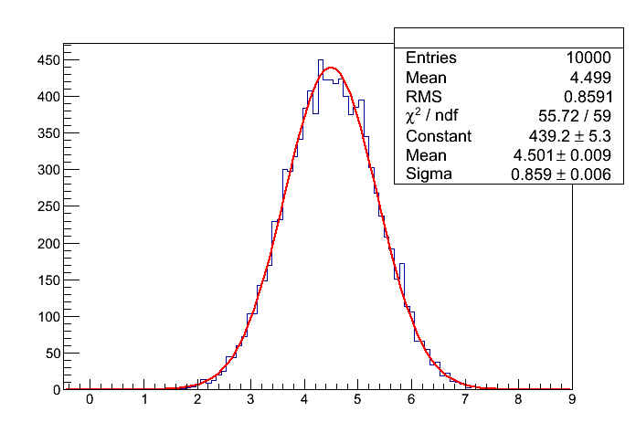
Result (example):
number of convoluted distributions = 9
chi2/ndf = 55.724/59 = 0.944475

