Lecture presented at the workshop
"Complex Systems in Natural and Social Sciences" (CSNSS’99),
14-17 September 1999, Kazimierz Dolny, Poland
To appear in Physical Review E 2000 |
Limits of time-delayed feedback control
Wolfram Just, Ekkehard Reibold, Hartmut Benner, Krzysztof
Kacperski, Piotr Fronczak, and Janusz Holyst
Max Planck Institute for Physics of Complex Systems, Nöthnitzer
Straß e 38, D-01187 Dresden, Germany
Institut für Festkörperphysik, Technische Universität
Darmstadt, Hochschulstraß e 6, D-64289 Darmstadt, Germany
Institute of Physics, Warsaw University of Technology,
Koszykowa 75, PL-00-662 Warsaw, Poland
e-mail: wolfram@mpipks-dresden.mpg.de
e-mail: Ekkehard.Reibold@physik.tu-darmstadt.de
e-mail: jholyst@if.pw.edu.pl
December 7, 1998
Abstract
General features of stability domains for time-delayed feedback control exist,
which can be predicted analytically. We clarify, why the control scheme with a
single delay term can only stabilise orbits with short periods or small Lyapunov
exponents, and derive a quantitative estimate. The limitation can be relaxed by
employing multiple delay terms. In particular, the extended time delay
autosynchronisation method is investigated in detail. Analytic calculations are
in good agreement with results of numerical simulations and with experimental
data from a nonlinear diode resonator.
Chaos control, Pyragas method, Differential-difference equation
1 Introduction
Controlling the motion of dynamical systems is one of the classical subjects in
engineering and mathematical science. Sophisticated tools have been developed
for that purpose (cf. e. g. []). Within the last decade such
topics have attracted the interest of many physicists in the context of
nonlinear dynamics since the potentially large number of unstable periodic
orbits which are embedded in chaotic attractors opens the possibility to
stabilise different states with very small control power. A conceptually quite
simple method which avoids fancy data processing and is based solely on the
plain measurement and the time lag of a scalar signal has been proposed by
Pyragas []. Despite the large amount of simulations and numerical analyses (cf. e. g. [,,,])
and several real experimental realisations (cf. [,]) little is known from
the theoretical and systematic point of view. Some progress has been made in
understanding topological constraints of the control scheme [,] and the
adaptation of delay times [] from a systematic point of view. Here, we are
concerned with the frequent numerical observation that the original Pyragas
method using a single delay time is limited to orbits with short periods or
small Lyapunov exponents. To overcome such limitations extended delay schemes
have been proposed [], but a deeper theoretical explanation is still missing.
2 Theoretical analysis
Following the lines of [] we start with a fairly general dynamical equation
which is subjected to a control force F,
We presuppose that without control, F ş 0,
the system admits an unstable periodic orbit x(t) = x(t+t)
with Floquet exponents ll+iwl.
At least one exponent has positive real part, l >
0. In what follows we concentrate on such a branch and, therefore, suppress the
subscript. The force aims at stabilising the orbit x.
Using the basic idea of delayed feedback control an appropriate force can be
derived simply from the measurement of a scalar quantity g[x(t)]
| F(t): = K |
Ą
ĺ
n = 0
|
sn {
g[x(t-nt)]
-g[x(t-(n+1)t)]}
. |
|
(2) |
Such a construction ensures that the periodic orbit remains a genuine
orbit of the system subjected to the control. The original method proposed by
Pyragas corresponds to the choice sn = dn,0,
whereas more general concepts like the extended time delay autosynchronisation
[] are also included by sn = Rn.
For convenience K denotes the control amplitude.
The stability of the periodic orbit is computed from the ordinary linear
stability analysis according to x(t) = x(t)+dx(t).
If we take into account that owing to the periodic time dependencies Floquet
theory can be applied [], i. e. dx(t)
= exp[(L+i W)t] v(t)
holds with Floquet exponent L+i W
and periodic eigenvectors v(t) = v(t+t),
we end up with
| L + i W
= G |
é
ë |
K { 1- exp[-(L+iW)t]} |
Ą
ĺ
n = 0
|
sn
exp[-n(L+iW)t] |
ů
ű |
. |
|
(3) |
The whole details of the system enter via a function G
which itself is a Floquet exponent determined by the linear stability of the
uncontrolled orbit and the control matrix []. In particular G[0]
= l+iw holds, G
is piecewise analytic and increases at most linearly with its argument. As
pointed out previously, a finite torsion is a necessary constraint for delayed
feedback methods to work at all (cf. [] for some rigorous statements).
Hence we restrict ourselves to the simplest case which is frequently met in
low-dimensional systems for topological reasons. We suppose namely that the
neighbourhood of the orbit flips during one turn, i. e. w
= p/t. In order to get
quantitative results we perform a Taylor series expansion of eq.(3).
Such an expansion can be performed at an arbitrary real value of the argument of
G. We obtain at first order, introducing
dimensionless quantities,
| P + i F = p -
x( 1+ exp[-P-iF]) |
Ą
ĺ
n = 0
|
(-1)n
sn exp[-(P+iF)n]
. |
|
(4) |
Here P = L t
denotes the Lyapunov exponent of the orbit subjected to control in units of the
period, F = Wt-p
the deviation of the frequency, x = (-tc˘)
K the rescaled control amplitude, and c˘
the real first Taylor series coefficient of G. If the
expansion is performed around zero, then p = G[0]t-ip
formally coincides with the Lyapunov exponent of the free orbit, lt.
For a different expansion point the value of p represents at least a first order
estimate for lt.
Henceforth we will identify p with the Lyapunov exponent of the free orbit. Both
quantities, c˘ as well as
p, depend explicitly on the details of the system and may be considered as fit
parameters. One might object that the approximation employed in eq.(4)
is too crude for studying real control properties. However, it has turned out
that several features can be predicted quite well even quantitatively [,].
Let us first recall the original Pyragas scheme, s0 = 1, sn
ł 1 = 0. For a given orbit the region of
stability, i. e. the parameter interval in x where eq.(4)
admits only solutions with P < 0, is typically bounded by two points. At the
lower boundary the real part L changes sign from
positive to negative values with a frequency W = w
= p/t, (F
= 0), i. e. a flip bifurcation occurs. On increasing the control
amplitude the stable eigenvalue branch collides with an additional exponent
giving rise to a finite frequency deviation F ą
0. The corresponding real part increases again and changes sign at the upper
bound of the stability interval causing a Hopf bifurcation. Both critical values
are easily evaluated from eq.(4) as
and
| x(ho) = F/sinF,
p = F/tan(F/2),
(F Î
[0,p]) , |
|
(6) |
where the second expression gives the parametric representation of the
boundary in the x-p plane. Fig. displays these boundaries in the parameter
plane. Although analytical calculations of such boundaries for fixed points of
the corresponding delay systems are well established (e. g. []) and
have been performed for particular maps and differential equations [] less has
been known about limit cycles. Here, we stress the fact that within our
approximation orbits with p > 2 cannot be stabilised at all. It is remarkable
that this critical value does not depend on the system parameter c˘.
Altogether our findings explain to some extent the frequent numerical
observation that orbits with large periods or highly unstable orbits cannot be
stabilised by the original Pyragas approach with a single delay term.
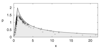
Figure 1: Stability domain for ordinary Pyragas control in the
parameter plane of rescaled control amplitude x and Lyapunov exponent p (greyshaded).
The solid/dashed line indicates the flip/Hopf instability (eq.(5)/(6)).
Symbols are results of simulations for the Rössler model with different
parameter settings.
Let us illustrate this analytical result with numerical simulations of the Rössler
model, [x\dot]1 = -x2-x3,
[x\dot]2 = x1+a x2, [x\dot]3 = b + x1
x3 -c x3. Using g[x] = x2
we have subtracted the control force (2) with sn
= dn, 0 from
the right hand side of the second equation. For control purpose we have focused
on the period-one orbit with respect to the canonical Poincaré surface of
section x1 = x2. Parameters have been chosen randomly from
the cube a Î [0.15,0.35], b Î
[0.1,0.8] and c Î [3,8]. For 100 parameter
combinations the minimal and maximal control amplitudes have been obtained from
plain time series like in real experimental situations. In each parameter
setting the delay time was adapted with a scheme similar to that proposed in [].
The Lyapunov exponent of the orbit was estimated by observing the exponential
escape from the orbit after switching off the control. The corresponding data
points are displayed in Fig. 1. To obtain the rescaled
control amplitude x the coefficient c˘
has been calculated for each orbit using the point of maximal stability []. The
coincidence between numerical data and the theoretical prediction is quite
convincing. Small deviations appear close to the critical value p = 2, since we
have not found unstable periodic orbits with p > 1.6.
3 Extended control schemes
To overcome the limitations which are caused by the size of the Lyapunov
exponent let us consider control schemes that employ multiple delay terms. For
the purpose of illustration we begin with the simplest extension by taking only
two delay terms into account, s0 = 1, s1 ą
0, sn ł 2 = 0.
Now the control scheme admits three parameters, the Lyapunov exponent of the
uncontrolled orbit p , the rescaled control amplitude x , and the relative
weight of the additional control term s1 . The stability boundaries
are caused by the same mechanism already described above. For the boundary
determined by the flip instability we obtain
whereas for the boundary generated by the Hopf instability eq.(4)
leads to
|
|
|
|
|
p
2
|
|
1+2 cosF
1+cosF
|
- |
F
sinF
|
|
2 cosF-1
2
|
|
|
|
|
|
|
ptan(F/2)-F
ptan(F/2)(1+2 cosF)
-F(2cosF-1)
|
, (F
Î [0,p])
. |
|
(8) |
|
|
|
Fig. shows the stability region determined by these curves for
three values of p. For p > 2 the stability region does not reach the x-axis,
i. e. stabilisation is not achieved by the original Pyragas scheme.
However, control is possible by employing the second delay term associated to
the variable s1. But even this method fails for p > 4 since the
stability domain vanishes, as easily computed from eqs.(7) and
(8).
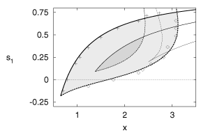
Figure 2: Stability boundaries for two time control in the
plane of rescaled control amplitude x and relative weight s1. Solid/dashed
lines indicate the flip/Hopf instability (eq.(7)/(8)).
Thick lines correspond to p = 1.53 and medium lines to p = 2.5. The stability
domains are shaded. In addition, the critical case p = 4.0 is shown by thin
lines. Crosses/diamonds indicate the results for the flip/Hopf boundary obtained
from a numerical simulation of the Rössler model using the values p = 1.53 and
(-tc˘)
= 0.88 for an optimal fit.
To confirm the analytical results, eqs.(7) and (8),
we used once more the Rössler model with parameter values a = b = 0.2 and c =
5.7. The control force was derived from the bounded quantity g[x] = tanh[(x1+x2)/10]
and the force was coupled to the first and the second equation of motion. The
stabilisation of the period-two orbit with period t =
11.758Ľ was considered. Within a straightforward
numerical simulation the domain in parameter space where stabilisation works
successfully was explored, and the data are displayed in Fig. 2.
Our data points are compared with the analytical results of eqs.(7)
and (8), where the unknown parameters p and (-tc˘)
have been fixed appropriately. The almost perfect agreement confirms that the
analytical results explain in the present case the main features not only
qualitatively, but even quantitatively.
Our previous considerations clearly show that the inclusion of additional
delay terms relaxes the constraint which originates from the size of the
Lyapunov exponent. Unfortunately, realising control forces with a large number
of independent delay terms becomes increasingly difficult. A very effective
control scheme which uses the advantage of multiple delays but is easily
implemented has been proposed in []. It corresponds to a geometrically
decreasing sequence of weights in eq. (2), sn
= Rn, |R|
< 1. According to eq.(4) the stability boundaries are
obtained as
and
|
|
|
|
| (p2 + F2) |
tan(F/2)
F+ptan(F/2)
|
|
|
|
|
|
|
p tan(F/2)-F
p tan(F/2)+F
|
, (F
Î [0,p])
. |
|
(10) |
|
|
|
Fig. shows the stability region for several values of R in the
x-p parameter plane as well as the stability region in the x-R control parameter
plane for different values of the Lyapunov exponent p.
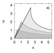
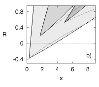
Figure 3: Stability boundaries for extended time delay
autosynchronisation : a) Parameter plane of rescaled control amplitude x and
Lyapunov exponent p with R = -0.3 (thin lines), R =
0.0 (medium lines), and R = 0.3 (thick lines); b) x-R control parameter plane
for three values of the Lyapunov exponent p (thick lines, from bottom to top p =
0.91, 2.89, 6.47). Solid/dashed lines indicate the flip/Hopf instability (eq.(9)/(10)),
the stability domains are shaded. Thin lines in b) display the numerically ''exact''
Hopf boundaries for the period-one orbit in the Rössler equation at a = 0.2,
0.6, and 0.9 with fit parameters (-tc˘)
= 0.33, 0.55, and 1.20 respectively (from bottom to top).
For each value of p there exists a finite stability interval in x, at least
if R is chosen sufficiently large. For fixed value of R the stability domains
extend up to a maximal p-value 2(1+R)/(1-R), as
easily computed from eqs.(9) and (10). By
employing large R-values control can always be achieved within our approximation.
In that sense the control scheme is superior to the ordinary Pyragas approach as
claimed in []. However, it follows from the analytical expressions that the
domain shrinks in size and shifts towards larger control amplitudes for
increasing values of the Lyapunov exponent p. Our analytical findings are in
agreement with the treatment of fixed points in two-dimensional systems [].
As in the previous case of two time delay we use the Rössler model to
illustrate our analytical result on extended control schemes. We concentrate on
the stabilisation of the period-one orbit at parameter values b = 0.2 and c =
5.7. Parameter a is varied to realise orbits with different Lyapunov exponents.
The stability boundaries within the K-R parameter plane can be computed ''exactly''
from the numerical solution of the linearised equation of motion. Such an
approach needs only the integration of plain differential equations (cf. []).
Results for three particular orbits, i. e. three particular system
parameters, are displayed in Fig. 3b. We stress that,
for appropriate values of the fit parameter p/(-tc˘),
the boundary caused by the flip instability coincides with the analytical
expression, since eq.(9) is an exact consequence of the full
eigenvalue equation (3) and valid beyond the first-order
Taylor series truncation. The deviations which occur for the boundary caused by
the Hopf instability can be attributed to such a simple approximation and hence
are not at all surprising. However, the qualitative features are correctly
reproduced. In addition, one should keep in mind that the exact Hopf boundary is
difficult to observe in plain simulations. Stabilisation is unlikely to occur in
the close vicinity of the transition line, because of finite basins of
attraction and small real parts, L.
Altogether our simple analytical expression captures most of the essential
features observed for the extended scheme. Last but not least, we mention that
the analytical formulas (9) and (10) are
again in reasonable agreement with the experimental data of [].
4 Electronic circuit experiments
Let us finally present results of the experiments performed on a nonlinear diode
resonator (cf. Fig. ). The circuit, consisting of a diode (1N4005), an
inductor (47 mH), and a resistor (36W), was
sinusoidally driven at fixed frequency (800 kHz).
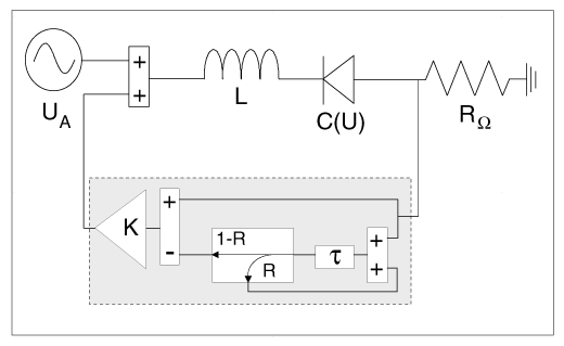
Figure 4: Experimental setup of the nonlinear diode resonator
with extended time delay feedback device.
Without control the system undergoes a period-doubling cascade into chaos on
variation of the driving amplitude UA. On further increase there
occur periodic windows of period-2, 3, 4, and 5 which also undergo
period-doubling cascades into chaos. Topological analysis [] of this
three-dimensional system yielded a frequency of p/ t
in the Floquet exponent for the unstable period-1, 2, and 4 orbits of the
chaotic attractor. This corresponds to a flip of the neighbourhood of these
orbits. Therefore, the orbits are accessible to time-delayed feedback control.
The control device consists of a cascade of electronic delay lines with a
limiting frequency of about 3 MHz and several operational amplifiers acting as
preamplifier, subtractor, or inverter. The device allows to apply a control
force of the form F(t) = - K [U(t) -
(1-R) S(t- t)],
S(t) = U(t) + R S(t- t)
which is equivalent to eq.(2) with sn
= Rn. Parameter ranges are R = 0Ľ1,
t = 10ns Ľ21 ms.
Our feedback scheme consisted of coupling the voltage at the resistor via the
control device to the driving force.
To check the coincidence with our analytical results for the simple and
extended control algorithm we measured the range of control amplitudes for
successful control of the period-one orbit and determined K(fl)
and K(ho) in dependence on the control
parameter R. The results for three different driving amplitudes are displayed in
Fig. .
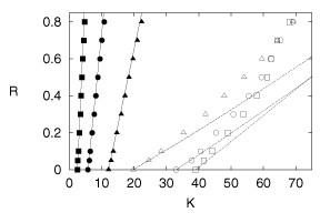
Figure 5: Stability range in the K-R parameter plane for three
values of the driving amplitude: [¯]
0.8V, ° 1.1V, \bigtriangleup 3.5V. Full/open symbols
corrspond to the flip/Hopf boundary. Solid/dashed lines indicate the analytical
result (9)/(10) with fit parameters [p;(-tc˘)]
= [0.69;0.137] (0.8V), [1.05;0.091] (1.1V), and [1.70;0.070] (3.5V).
The fit of the analytical result yields a perfect agreement for the flip
boundary, for the reason already mentioned above. As expected, we observe slight
deviations for the Hopf boundary since the analytical result is just a
first-order approximation.
In addition, we measured the Lyapunov exponent of the free orbit, p, by
observing the exponential increase of the control signal when the control is
turned off. The frequency deviation F can be measured
with high precision from the spectrum of the control signal at the Hopf boundary,
whereas exponents p larger than one are difficult to evaluate from the
experimental data. The experimental stability boundaries in the K-p parameter
plane as well as the corresponding values of the frequency deviation are shown
in Fig. .
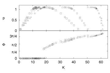
Figure 6: Stability boundaries in the K-p plane for the
period-one orbit and corresponding frequency deviation F
for three values of R: [¯] (R =
0), ° (R = 0.2), and \bigtriangleup (R = 0.5)
obtained from the transient dynamics in the electronic circuit experiment.
Although one observes a qualitative agreement with the corresponding
analytical result (cf. Fig. 3a), a quantitative
evaluation is difficult to perform. For each data point one has at least one fit
parameter (-tc˘)
so that at this level no real comparison can be made. Fortunately eqs.(9)
and (10) yield a relation between the two critical amplitudes
K(fl), K(ho),
the control parameter R, and the frequency deviation at the Hopf boundary F
which does not contain any system parameter
|
K(fl)
K(ho)
|
= 1 |
/ |
|
é
ę
ë |
1+ |
ć
ç
č |
1-R
1+R
|
tan |
F
2
|
ö
÷
ř |
2
|
ů
ú
ű |
. |
|
(11) |
Although we could already compare this expression with the data
presented in Fig. 6, the accessible range of
frequency deviations is too small for meaningful results. Therefore we
concentrate on control of the period-4 orbit and the corresponding data are
shown in Fig. . In view of the fact that the analytical curves do not
contain any fit parameter the coincidence is remarkable. Hence, we conclude that
already the first order analytical expression contains the essential qualitative
and several quantitative features which determine the stability domain for
feedback control.
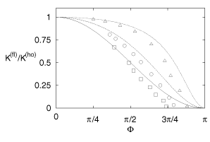
Figure 7: Ratio of critical control amplitudes in dependence on
the frequency deviation F at the Hopf instability for
several values of R. Symbols are results of the electronic circuit experiment,
lines display the analytical expression (11): R = 0 ([¯],
solid line), R = 0.2 (°, dashed line), and R = 0.5
(\bigtriangleup, dotted line).
5 Conclusion
In conclusion, our analytical approach, which was based on a first-order series
expansion in the control amplitude has shown that the collision of eigenvalues
resulting in a finite frequency deviation limits the success of time-delayed
feedback control. Within our approximation the original Pyragas scheme is
limited to orbits with short periods or small Lyapunov exponents such that lt
< 2. The limitation can be overcome by taking multiple delays into account.
The inclusion of two delay terms relaxes the condition to lt
< 4, while for the extended time delay autosynchronisation in principle no
constraint is obtained at this level. For all schemes there are limited ranges
of the control amplitude K that can be employed to stabilise the desired
periodic orbit, and orbits with large values of the exponent lt
can be stabilised only in very limited ranges of K.
Our analytical approach was restricted to a first-order approximation. Of
course, one cannot expect that the shape of control domains is always reproduced
to a high accuracy since the details depend on the system under consideration.
Moreover one should keep in mind that in particular for large control amplitudes
nonlinear contributions from the eigenvalue equation may become important, which
might result in the appearance of new stability regions as well as a deformation
of those domains predicted by the linear theory (cf. []). However, we found
at least qualitative coincidence in our numerical and experimental
investigations. In addition, we stress that quite similar features have been
observed in different experimental realisations []. There, the control domain is
often considered in terms of the actual system parameters and not in terms of
the Lyapunov exponent of the orbit. In order to compare with our analytical
result one has also to take into account the nonlinear dependence of the
Lyapunov exponent on the system parameters.
Concerning the analysis of control domains we have focused on the
eigenbranches associated with one positive exponent of the unstable orbit. In
general, these domains may be further limited e. g. by other
eigenbranches which are connected to the stable exponents of the uncontrolled
orbit and may become unstable in the course of control. Although these features
are captured by our approximate analytical treatment, they depend on the
particular system under consideration, since additional fit parameters enter.
Above all, the results of our analytic calculations are in reasonable
agreement with numerical simulations and experimental data of an electronic
circuit so that the theoretical approach captures most of the essential features.
Acknowledgement
This project of SFB 185 ''Nichtlineare Dynamik'' was partly financed by special
funds of the Deutsche Forschungsgemeinschaft. We are indebted to F. Laeri
and M. Müller for the use of their delayed feedback control device.
References
- []
- R. Bellman, Adaptive Control Processes: A Guided Tour, (Princeton
Univ. Press, Princeton, 1961).
- []
- K. Pyragas, Phys. Lett. A 170, 421 (1992).
- []
- K. Pyragas and A. Tamasevicius, Phys. Lett. A 180,
99 (1993).
- []
- D. J. Gauthier, D. W. Sukow, H. M. Concannon,
and J. E. S. Socolar, Phys. Rev. E 50, 2343
(1994).
- []
- J. E. S. Socolar, D. W. Sukow, and D. J. Gauthier,
Phys. Rev. E 50, 3245 (1994).
- []
- K. Pyragas, Phys. Lett. A 206, 323 (1995).
- []
- S. Bielawski, D. Derozier, and P. Glorieux, Phys. Rev. E
49, R971 (1994).
- []
- T. Pierre, G. Bonhomme, and A. Atipo, Phys. Rev. Lett. 76,
2290 (1996)
- []
- W. Just, T. Bernard, M. Ostheimer, E. Reibold, and H. Benner,
Phys. Rev. Lett. 78, 203 (1997).
- []
- H. Nakajima, Phys. Lett. A 232, 207 (1997).
- []
- W. Just, D. Reckwerth, J. Möckel, E. Reibold, and H. Benner,
Phys. Rev. Lett. 81, 562 (1998)
- []
- J. K. Hale and S. M. Verduyn Lunel, Introduction to
Functional Differential Equations (Springer, New York, 1993).
- []
- L. Collatz, Z. angew. Math. Mech. 25/27,
60 (1947)
- []
- A. Kittel, J. Parisi, and K. Pyragas, Phys. Lett. A
198, 433 (1995)
- []
- M. E. Bleich and J. E. S. Socolar, Phys. Lett. A
210, 87 (1996).
- []
- D. Sukow, M. E. Bleich, D. J. Gauthier, and J. E. S. Socolar,
Chaos 7, 560 (1997).
- []
- N. B. Tufillaro, T. Abbott, and J. Reilly, An
Experimental Approach to Nonlinear Dynamics and Chaos (Addison-Wesley,
Redwood, 1992)
Footnotes:
1[
2[
3[
File translated from TEX by TTH,
version 2.55.
On 18 Jan 2000, 09:48.